Earthviewer
04.12.2015 21:52 by chris
Earthviewer is a small project, which renders a moving model of the Earth using a bunch of textures and some other cg tricks. Currently I am implementing atmospheric scattering.
Dieses Video sowie der folgende Download basieren auf Revision EEAA90CE.
Earthviewer Download
Visual C++ x86 Runtime Try to install this, if there is an error message while starting.
Appreciation
06.12.2015 17:46 by chris
When creating Earthviewer, I used a bunch of free libraries and assets. Here are the most important ones:
Libs
- Open Asset Import Library: 3D model import library
- Simple and Fast Multimedia Library: Multimedia framework, used for OpenGL context creation and window event handling
- AntTweakBar: Provides an easy way of creating a small GUI for tweaking variables. I used it as a debug tool for viewing variable values at runtime.
Assets
- Natural Earth III: Earth image data, going from texture maps to elevation maps. I used a night texture, a cloud map and the land/water mask.
- NASA Visible Earth – The Blue Marble: This is where the day texture is from and I also used one of their Bathymetry maps.
- Ponies & Light Normal Map: The personal blog of @tgfrerer, he wrote an article about extracting normal maps from elevation data. I used his results in my project.
- Milky Way Skybox Textures: Originally made for Kerbal Space Program using Space Engine. Unfortunately I do not know the author because of his reddit and mediafire account being deleted.
I also want to appreciate some tutorials which helped me alot:
Tutorials
- Wikibooks Arcball Camera
- Rastergrid – Efficient Gaussian blur with linear sampling
- Philip Rideout – OpenGL Bloom Tutorial
Ray-Sphere Intersection
10.01.2018 19:02 by chris
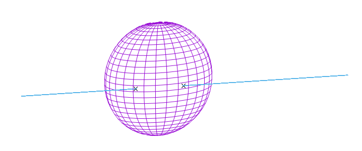
When developing atmospheric scattering shaders, we will need to calculate intersection points between rays and spheres. So here is how we can do that.
Defining a ray
To define a ray, we specify two vectors: One point o, which goes from zero to a point on the ray and another one d, which goes along the ray and defines therefore the ray’s direction. The direction vector is multiplied by an argument t. When varying t, we can reach any point on the ray. Now you might say, that we did not define a ray, but a line. The only difference between rays and lines is, that t has a minimum value for rays. A line goes from -infinity to infinity, while a ray has a starting point and goes to infinity from there. In our use case, that’s not that important tough.

Defining a sphere
To define a sphere, we need to specify a center point c and a radius r. All points on a sphere are points, which have a distance to the center point equally to the sphere’s radius. So a sphere’s definition can be: 

Intersecting both
In our use case, we will have the spheres always centered, so we can use the easier version of the sphere definition. Inserting the ray definition into the sphere definition yields:


Image a vector 

From the definition of the dot product and
So there is


To apply this to the intersection, we need to square it first:

\cdot(\overrightarrow{o}+t_{\mathrm{hit}}\overrightarrow{d})")
^2 =\overrightarrow{o}^2+2\overrightarrow{o}\cdot\overrightarrow{d}t_{\mathrm{hit}}+\overrightarrow{d}^2t_{\mathrm{hit}}^2")


To make the calculation easier we assume, that 

Now we use the reduced quadratic formula to solve the equation for
The discriminant is
So the cheapest way to calculate the intersection point is:

^2-q")

^2-\overrightarrow{o}^2+r^2}")
^2-\overrightarrow{o}^2+r^2}")


Keep in mind, that 
Numerical Integration
06.01.2018 06:17 by chris
To describe atmospheric scattering, we will use several equations with integrals which can’t be solved analytically – so we will make use of middle Riemann sums to approximate those.
Image a function f which can’t be integrated analytically. It might have a function graph like this:
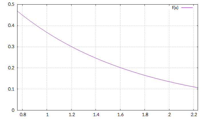
In this case it is the graph for =e^{-x}")
Let’s say, we want to integrate it from x=1 to x=2: 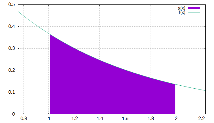
To calculate this integral, we will divide the complete integral into n intervals and approximate each part with a rectangle, for example n=3:

When the bounds are a und b, each interval has a width of:

Next we need the height of each rectangle. Here there are several possibilities to choose from, we use the value of our function in the middle of each interval (that’s why it is called middle sum):
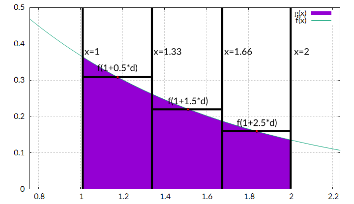
Now we can calculate the area of each rectangle:
\mathrm{d})")
[table]
i,a+(i+0.5)d,f(a+(i+0.5)d),Ai
0,1.16666666666667,0.311403223914598,0.103801074638199
1,1.5,0.22313016014843,0.074376720049477
2,1.83333333333333,0.159879746079694,0.053293248693231
[/table]
Adding all rectangles yields:

Let’s check:
![\displaystyle\int_1^2 e^{-x}= \left[ -e^{-x} \right]_1^2 = -e^{-2}+e^{-1}=\frac{1}{e}-\frac{1}{e^2}=\frac{e}{e^2}-\frac{1}{e^2}](https://s0.wp.com/latex.php?latex=%5Cdisplaystyle%5Cint_1%5E2+e%5E%7B-x%7D%3D+%5Cleft%5B+-e%5E%7B-x%7D+%5Cright%5D_1%5E2+%3D+-e%5E%7B-2%7D%2Be%5E%7B-1%7D%3D%5Cfrac%7B1%7D%7Be%7D-%5Cfrac%7B1%7D%7Be%5E2%7D%3D%5Cfrac%7Be%7D%7Be%5E2%7D-%5Cfrac%7B1%7D%7Be%5E2%7D&bg=ffffff&fg=000000&s=1 "\displaystyle\int_1^2 e^{-x}= \left[ -e^{-x} \right]_1^2 = -e^{-2}+e^{-1}=\frac{1}{e}-\frac{1}{e^2}=\frac{e}{e^2}-\frac{1}{e^2}")

In this case there is an error of 0.46606%, pretty good for just using three sample intervals. When using more samples, the approximation gets more accurate, here are the results when using 3, 10, 50 and 500 samples:
[table]
n,Approximation,Error
3,0.231471043380907,0.461467 %
10,0.232447292788817,0.041655 %
50,0.232540282244081,0.001667 %
500,0.232544119177475,0.000017 %
[/table]
There is a lot of theory for quantifying the error, but I will omit it here. All we will need is the following equation for numeric integration by middle Riemann sums:
\,dx \approx \frac{b-a}{n}\sum_{i=0}^{n-1} f\left(a+\left(\frac{1}{2}+i\right)\frac{b-a}{n}\right)")