Numerical Integration
06.01.2018 06:17 by chris
To describe atmospheric scattering, we will use several equations with integrals which can’t be solved analytically – so we will make use of middle Riemann sums to approximate those.
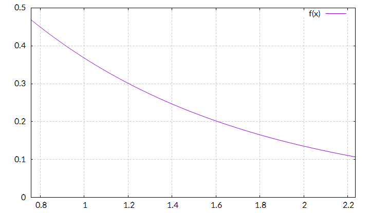
Image a function f which can’t be integrated analytically. It might have a function graph like this:

In this case it is the graph for , which is important for atmospheric scattering. Of course, we can integrate it directly, but we will use this function anyway, so that we can compare our approximation with the direct result.
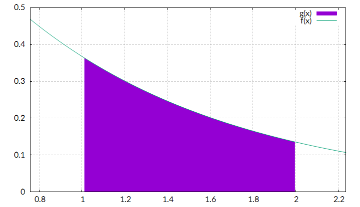
Let’s say, we want to integrate it from x=1 to x=2: 
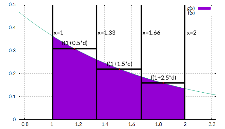
To calculate this integral, we will divide the complete integral into n intervals and approximate each part with a rectangle, for example n=3:

When the bounds are a und b, each interval has a width of:
Next we need the height of each rectangle. Here there are several possibilities to choose from, we use the value of our function in the middle of each interval (that’s why it is called middle sum):

Now we can calculate the area of each rectangle:
[table]
i,a+(i+0.5)d,f(a+(i+0.5)d),Ai
0,1.16666666666667,0.311403223914598,0.103801074638199
1,1.5,0.22313016014843,0.074376720049477
2,1.83333333333333,0.159879746079694,0.053293248693231
[/table]
Adding all rectangles yields:
Let’s check:
In this case there is an error of 0.46606%, pretty good for just using three sample intervals. When using more samples, the approximation gets more accurate, here are the results when using 3, 10, 50 and 500 samples:
[table]
n,Approximation,Error
3,0.231471043380907,0.461467 %
10,0.232447292788817,0.041655 %
50,0.232540282244081,0.001667 %
500,0.232544119177475,0.000017 %
[/table]
There is a lot of theory for quantifying the error, but I will omit it here. All we will need is the following equation for numeric integration by middle Riemann sums: